北邮Matlab选修 Week 12 拟合

拟合函数

问题描述

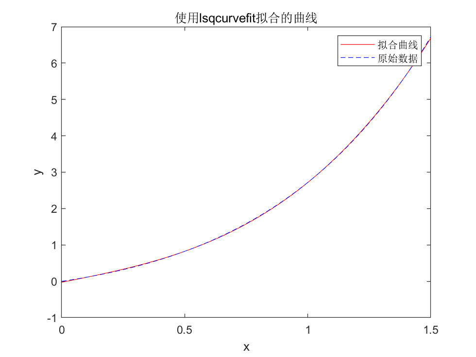
设$f(x)=xe^x,x \in [0,1.5]$，求$f(x)$的三次近似最佳平方逼近多项式。

程序设计

 1
 2
 3
 4
 5
 6
 7
 8
 9
10
11
12
13
14
15
16
17
18
19
20
21


%question1.m
x0=[10;10;10;10];%初始参数猜测值
xdata=linspace(0,1.5,5000);%生成x数据点
ydata=xdata.*exp(xdata);%生成对应的y数据点
%定义函数模型
fun=@(x,xdata)x(1)*xdata.^3+x(2)*xdata.^2+x(3)*xdata+x(4);

[x,resnorm]=lsqcurvefit(fun,x0,xdata,ydata);

%打印出拟合的参数
disp(['拟合的参数:a=',num2str(x(1)),',b=',num2str(x(2)),',c=',num2str(x(3)),',d=',num2str(x(4))]);
disp(['拟合的方程:',num2str(x(1)),'*x^3+',num2str(x(2)),'*x^2+',num2str(x(3)),'*x+',num2str(x(4))]);

%绘制图形
plot(xdata,fun(x,xdata),'r-',xdata,ydata,'b--');

%添加图例和标题
legend('拟合曲线','原始数据');
title('使用lsqcurvefit拟合的曲线');
xlabel('x');
ylabel('y');

计算结果

1
2
3


>> question1
拟合的参数:a=1.3877,b=-0.0047124,c=1.3623,d=-0.028475
拟合的方程:1.3877*x^3+-0.0047124*x^2+1.3623*x+-0.028475

计算参数

问题描述

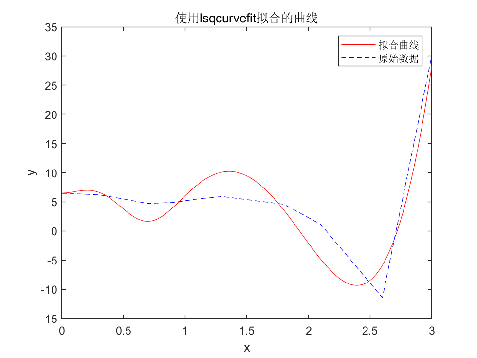
已知一组观测数据$(x_i,y_i)$见下表，函数的原型为$y=a_1+a_2x^2+a_3e^{-5x^3}+a_4cos(-2x)+a_5x^4$，试用所给数据求出待定系数$a_i$的值。

$x_i$	$y_i$	$x_i$	$y_i$
0	6.3700	1.1	5.4941
0.1	6.3888	1.3	5.9187
0.3	6.2056	1.8	4.5944
0.4	5.8676	2.1	1.1440
0.7	4.7256	2.6	-11.4326
0.9	4.8990	3.0	30.0009
0.95	5.0383

程序设计

 1
 2
 3
 4
 5
 6
 7
 8
 9
10
11
12
13
14
15
16
17
18
19
20
21


%question2.m
x0=[10;10;10;10;10];%初始参数猜测值
x1=linspace(0,3,5000);%生成x数据点
xdata=[0;0.1;0.3;0.4;0.7;0.9;0.95;1.1;1.3;1.8;2.1;2.6;3.0];%生成x数据点
ydata=[6.3700;6.3888;6.2056;5.8676;4.7256;4.8990;5.0383;5.4941;5.9187;4.5944;1.1440;-11.4326;30.0009];%生成对应的y数据点
%定义函数模型
fun=@(x,xdata)x(1)+x(2)*xdata.^2+x(3)*exp(-5*xdata.^3)+x(4)*cos(-2*xdata)+x(5)*xdata.^4;

[x,resnorm]=lsqcurvefit(fun,x0,xdata,ydata);

%打印出拟合的参数
disp(['拟合的参数:a1=',num2str(x(1)),',a2=',num2str(x(2)),',a3=',num2str(x(3)),',a4=',num2str(x(4)),',a5=',num2str(x(5))]);

%绘制图形
plot(x1,fun(x,x1),'r-',xdata,ydata,'b--');

%添加图例和标题
legend('拟合曲线','原始数据');
title('使用lsqcurvefit拟合的曲线');
xlabel('x');
ylabel('y');

计算结果

1
2


>> question2
拟合的参数:a1=9.4777,a2=-16.5136,a3=22.4145,a4=-25.3911,a5=2.3676

面积计算

问题描述

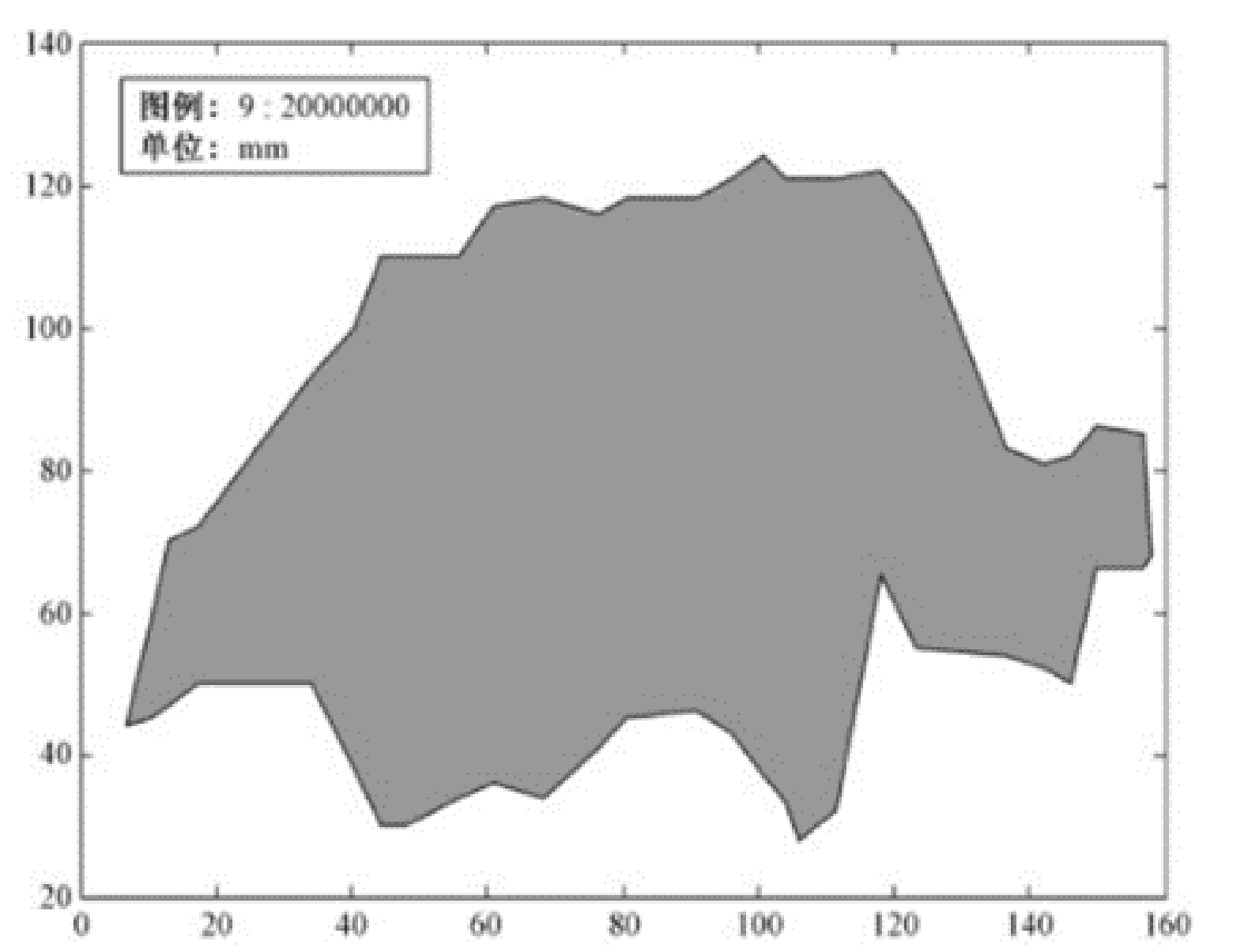
已知欧洲某个国家的地图如下图所示，为了计算出它的国土面积，首先对地图进行如下测量：以由西向东方为$x$轴，由南向北方为$y$轴，选择方便的原点，并将从最西边界点到最东边界点在$x$轴上的区间适当的分成若干段，在每个点的$y$方向测出南边界点和北边界点的$y$坐标$y_1$和$y_2$，这样就得到了表中所示的测量数据（单位：mm）。 map

$x$	$y_1$	$y_2$	$x$	$y_1$	$y_2$	$x$	$y_1$	$y_2$
7.0	44	44	61	36	117	111.5	32	121
10.5	45	59	68.5	34	118	118	65	122
13.0	47	70	76.5	41	116	123.5	55	116
17.5	50	72	80.5	45	118	136.5	54	83
34	50	93	91	46	118	142	52	81
40.5	38	100	96	43	121	146	50	82
44.5	30	110	101	37	124	150	66	86
48	30	110	104	33	121	157	66	85
56	34	110	106	28	121	158	68	68

数学模型

事实上，由图像不难看出，该国家的国土面积实际上是由$y_1=f_1(x)$和$y_2=f_2(x)$两条曲线包围起来的。因此，我们只需要求解$f_1(x)$和$f_2(x)$，然后通过积分$\int\limits_{7.0}^{56}(f_2(x)-f_1(x))dx $就可以得到。

程序设计

 1
 2
 3
 4
 5
 6
 7
 8
 9
10
11
12
13
14
15


%question3.m
%定义初始值
x=[7.0,10.5,13.0,17.5,34,40.5,44.5,48,56,61,68.5,76.5,80.5,91,96,101,104,106,111.5,118,123.5,136.5,142,146,150,157,158];
y1=[44,45,47,50,50,38,30,30,34,36,34,41,45,46,43,37,33,28,32,65,55,54,52,50,66,66,68];
y2=[44,59,70,72,93,100,110,110,110,117,118,116,118,118,121,124,121,121,121,122,116,83,81,82,86,85,68];
%定义微分间隔
d=0.01;
dx=7:d:158;
%插值
y1_=interp1(x,y1,dx,'linear');
y2_=interp1(x,y2,dx,'linear');
s=sum(y2_-y1_)*d/18^2*1600;
%输出结果
fprintf('The sum of the differences between the two curves is %.2f km^2\n',s);
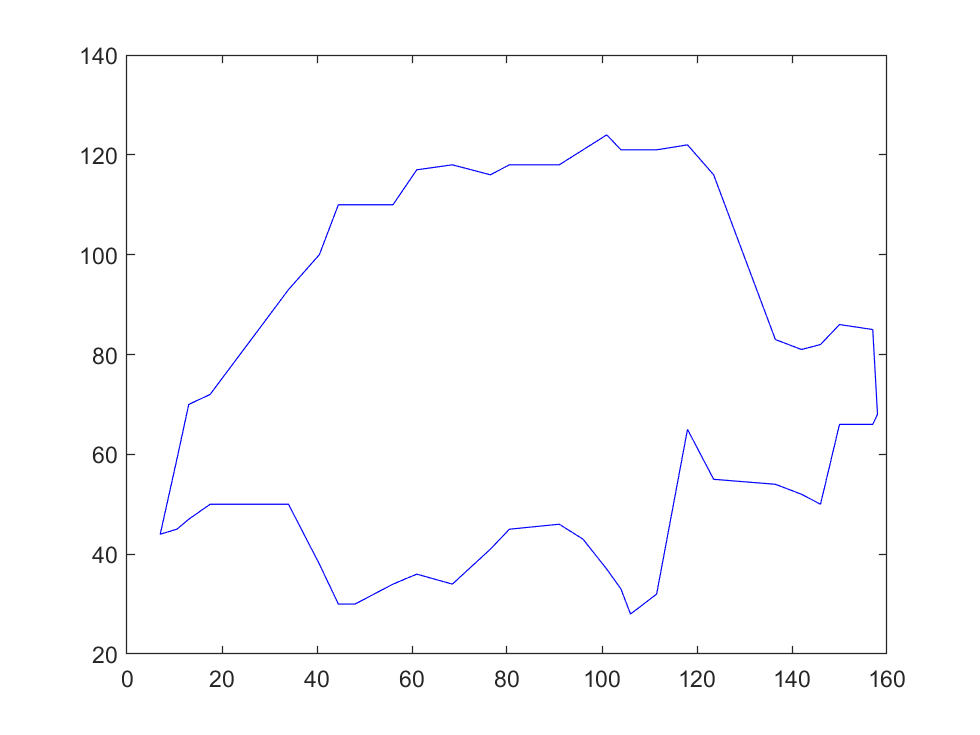
plot(x,y1,'b',x,y2,'b');

计算结果

1
2


>> question3
The sum of the differences between the two curves is 42414.81 km^2

第十二周作业-拟合

BUPT大一下Matlab选修

北邮Matlab选修 Week 12 拟合

拟合函数

问题描述

程序设计

计算结果

计算参数

问题描述

程序设计

计算结果

面积计算

问题描述

数学模型

程序设计

计算结果